20+ Excel Functions for Data Analysis: A Practical Guide With Examples
By William DavisSeptember 27, 2026
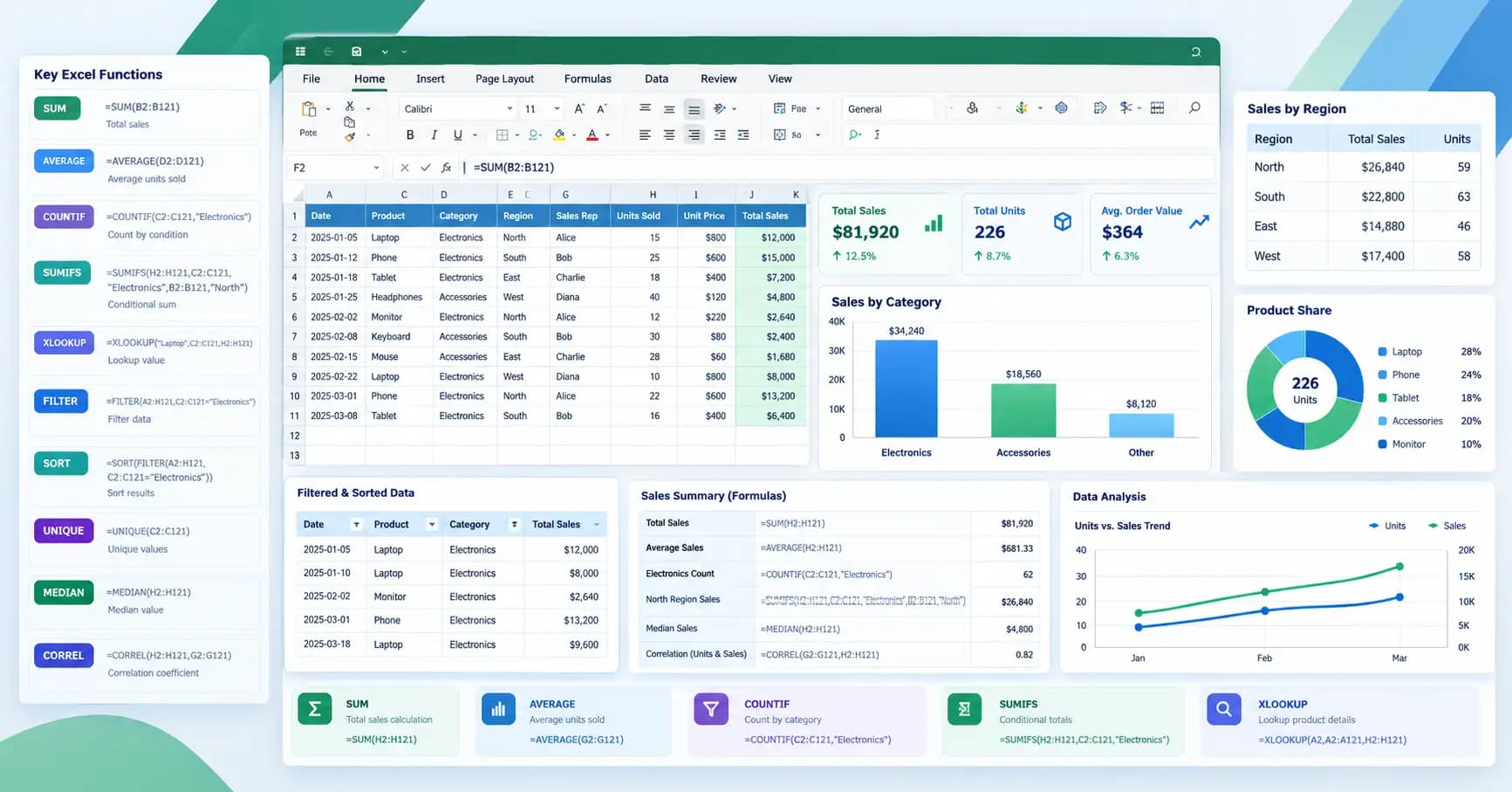
Excel is still one of the most useful tools for working with data. You can use it to clean raw records, find totals, compare groups, rank results, spot trends, and build reports without writing code. Excel functions make these jobs faster by applying ready-made calculations to your data. Industry data analytics curricula and official spreadsheet documentation consistently highlight functions such as SUM, AVERAGE, IF, COUNTIF, SUMIF, XLOOKUP, and text functions as essential tools for daily analytical work.
The hard part isn't knowing that Excel has hundreds of functions. The real challenge is knowing which ones to use and when.
This guide covers more than 20 Excel functions for data analysis, with simple examples you can try on a sales, finance, survey, customer, or operations dataset.
What Are Excel Functions for Data Analysis?
Excel functions are built-in formulas that take your data as input and return a result. They can add numbers, calculate averages, count records, test conditions, find matching values, clean text, and return filtered lists.
For example, suppose your worksheet has:
| Date | Region | Product | Units | Revenue |
|---|---|---|---|---|
| 01/09/2026 | North | Laptop | 5 | 5000 |
| 02/09/2026 | South | Monitor | 8 | 2400 |
| 03/09/2026 | North | Laptop | 3 | 3000 |
You can use Excel functions to answer questions such as:
How much revenue did we make?
What was the average sale?
Which region made the most money?
How many orders were over $1,000?
Which customers bought a certain product?
Are two sets of data related?
Which values are unusual?
How can I clean messy imported data?
Let's look at the functions that help answer these questions.
1. SUM
SUM adds numbers from cells or ranges. It's one of the most common functions in Excel and a useful starting point for data analysis.
Syntax:
=SUM(E2:E100)This adds all revenue values from E2 to E100.
You can use it to calculate total sales, total costs, total units, monthly income, or any other numeric total.
2. AVERAGE
AVERAGE returns the arithmetic mean of a group of numbers.
=AVERAGE(E2:E100)For a sales report, this can tell you the average revenue per record.
Remember that the mean can be affected by very large or very small values. For uneven data, MEDIAN may give you a more useful view.
3. MEDIAN
MEDIAN finds the middle value in a set of numbers after the values are arranged in order.
=MEDIAN(E2:E100)Imagine most customer orders are between $50 and $200, but one order is $20,000. The average could rise sharply, while the median can still show the typical order more clearly.
Median is useful for income data, order values, delivery times, and customer spending.
4. MIN
MIN returns the smallest number in a range.
=MIN(E2:E100)You can use it to find the lowest sale, smallest order, minimum response time, or lowest monthly value.
5. MAX
MAX returns the largest value in a range.
=MAX(E2:E100)For a sales dataset, MAX can show the largest order or highest recorded revenue.
Using MIN and MAX together gives you a quick view of the spread between the lowest and highest values.
6. COUNT
COUNT counts cells that contain numbers.
=COUNT(E2:E100)This is useful when you need to know how many numeric records are present in a column.
For example, you may have 100 rows but only 94 rows with valid revenue values. COUNT helps reveal that difference.
7. COUNTA
COUNTA counts cells that aren't empty.
=COUNTA(A2:A100)Unlike COUNT, it can count text as well as numbers.
This makes it useful for checking how many customer names, product names, or order IDs have been entered.
8. COUNTIF
COUNTIF counts cells that meet one condition.
=COUNTIF(B2:B100,"North")This counts records where the region is North.
You can also use number conditions:
=COUNTIF(E2:E100,">1000")That counts sales above 1,000.
COUNTIF is handy when you need a quick answer about how often something happens.
9. COUNTIFS
COUNTIFS counts records that meet multiple conditions. Microsoft lists it among Excel's statistical functions for counting values against more than one criterion.
=COUNTIFS(B2:B100,"North",E2:E100,">1000")This counts rows where the region is North and revenue is above 1,000.
It's useful when a simple COUNTIF isn't enough.
10. SUMIF
SUMIF adds values that meet one condition.
=SUMIF(B2:B100,"North",E2:E100)This adds revenue for the North region.
You could use the same idea to calculate sales for one product, one salesperson, or one customer group.
11. SUMIFS
SUMIFS adds values that meet multiple conditions. Microsoft describes it as a function for summing values when several criteria are met.
=SUMIFS(E2:E100,B2:B100,"North",C2:C100,"Laptop")This returns revenue from Laptop sales in the North region.
This is one of the most useful functions when working with transaction data because you can combine several filters inside one formula.
12. AVERAGEIF
AVERAGEIF calculates the average for cells that meet a condition.
=AVERAGEIF(B2:B100,"North",E2:E100)This returns the average revenue for North.
You can use it to compare the average order value across regions, products, teams, or other groups.
13. IF
IF checks a condition and returns one result when it is TRUE and another when it is FALSE. Microsoft describes it as a core logical function for making comparisons.
=IF(E2>=1000,"High","Low")This classifies each sale as High or Low.
You can use IF to create useful analysis columns such as:
=IF(D2>=10,"Target Met","Below Target")This is useful when turning raw numbers into categories that are easier to read.
14. IFERROR
Formulas don't always return the result you expect. IFERROR lets you replace an Excel error with your own value.
=IFERROR(E2/D2,0)If D2 is zero and the division would return an error, Excel shows 0 instead.
For reports, this can keep error messages from filling your output with values such as #DIV/0! or #N/A.
15. XLOOKUP
XLOOKUP searches one range and returns a related value from another range. It can search in different directions and uses exact match by default. Microsoft lists it as an improved lookup option over older lookup methods.
=XLOOKUP(H2,A2:A100,E2:E100,"Not Found")Suppose H2 contains an order ID. The formula searches column A and returns the related revenue from column E.
This is useful for customer records, product lists, employee data, invoices, and sales tables.
Version note: Microsoft says XLOOKUP isn't available in Excel 2016 or Excel 2019, even though newer workbooks using it may open in those versions.
16. INDEX
INDEX returns a value from a range based on its position.
=INDEX(E2:E100,5)This returns the fifth value from E2:E100.
INDEX is often paired with MATCH for more flexible lookups.
17. MATCH
MATCH returns the position of a value within a range.
=MATCH(H2,A2:A100,0)The 0 asks Excel for an exact match.
You can combine INDEX and MATCH like this:
=INDEX(E2:E100,MATCH(H2,A2:A100,0))This approach has been widely used for table lookups, including in financial models and reporting workbooks.
18. FILTER
FILTER returns rows that meet a condition. It is especially useful when you want a live result rather than changing the original table. Microsoft documents FILTER as a dynamic array function that filters data using TRUE or FALSE conditions.
=FILTER(A2:E100,B2:B100="North","No records")This returns all rows from the North region.
You can also combine conditions:
=FILTER(A2:E100,(B2:B100="North")*(E2:E100>1000),"No records")Now Excel returns rows where the region is North and revenue is above 1,000.
19. SORT
SORT arranges the contents of a range or array in ascending or descending order.
=SORT(A2:E100,5,-1)Here, Excel sorts the data using the fifth column in descending order.
This is helpful when you want to create a live top-sales list without manually sorting the source table.
You can also combine it with FILTER:
=SORT(FILTER(A2:E100,B2:B100="North"),5,-1)That gives you North region sales sorted from highest to lowest.
20. UNIQUE
UNIQUE returns a list of distinct values from a range.
=UNIQUE(C2:C100)This creates a list of unique products.
You can combine UNIQUE with SORT:
=SORT(UNIQUE(C2:C100))That gives you a clean alphabetical product list. Microsoft also shows SORT and UNIQUE being used together for this type of result.
21. SUMPRODUCT
SUMPRODUCT multiplies matching values in arrays and then adds the results. It can also perform other arithmetic with array values.
Suppose D contains units sold and F contains unit price:
=SUMPRODUCT(D2:D100,F2:F100)This calculates total revenue by multiplying each row's units by its price and then adding the results.
SUMPRODUCT also works well for analysis with several conditions without adding helper columns.
22. TRIM
Raw data often contains extra spaces. TRIM removes extra spaces except for single spaces between words.
=TRIM(A2)For example, a value such as:
John Smithcan become:
John SmithThis matters because messy spaces can cause matching and lookup problems.
One limitation is worth knowing. Microsoft notes that TRIM does not remove the nonbreaking space character often found in copied web data by itself.
23. LEFT
LEFT returns characters from the start of a text string.
=LEFT(A2,3)If A2 contains ORD-2589, the result is ORD.
This can help extract order prefixes, region codes, or other text-based IDs.
24. RIGHT
RIGHT returns characters from the end of a text string.
=RIGHT(A2,4)For ORD-2589, this returns 2589.
It's useful when IDs or codes place useful information at the end of the text.
25. MID
MID extracts characters from the middle of a string based on a starting position and number of characters.
=MID(A2,5,4)This can help pull a section from a long product code or reference number.
LEFT, RIGHT, and MID are often used during the data-cleaning stage.
26. TEXTSPLIT
TEXTSPLIT breaks text into separate cells using a delimiter. Microsoft describes it as the formula-based version of Excel's Text to Columns feature.
=TEXTSPLIT(A2,",")If A2 contains:
Laptop,North,5000Excel can split it into separate cells.
This is useful when imported data stores several fields in one cell.
TEXTSPLIT is available in newer Excel versions, including Microsoft 365 and Excel 2024.
27. TEXTJOIN
TEXTJOIN combines text from several cells and places a delimiter between each value.
=TEXTJOIN(", ",TRUE,A2:A5)This can turn separate values into one readable line.
For example:
Laptop
Monitor
Keyboard
Mouse
can become:
Laptop, Monitor, Keyboard, MouseThis is useful when creating summaries or combining cleaned fields.
28. RANK.EQ
RANK.EQ returns the rank of a number compared with other values in a list. Microsoft says it assigns the same rank to tied values and gives the top rank to the tied group.
=RANK.EQ(E2,$E$2:$E$100,0)This ranks each sale from highest to lowest.
For sales dashboards, performance reports, and contest data, ranking can make comparisons much easier.
29. QUARTILE.INC
QUARTILE.INC returns quartile values from a dataset. Quartiles split a set of numbers into useful sections, such as the bottom 25% and top 25%.
=QUARTILE.INC(E2:E100,1)This returns the first quartile.
You can use it to study income, sales, scores, delivery time, or customer spending.
Microsoft recommends the newer QUARTILE.INC and QUARTILE.EXC functions instead of the older QUARTILE function for new work.
30. STDEV.S
STDEV.S estimates standard deviation for a sample. Standard deviation shows how widely values vary around the mean.
=STDEV.S(E2:E100)A low result suggests the values are closer to the average. A higher result means the data is more spread out.
Use STDEV.P when your data represents the full population rather than a sample. Microsoft makes this distinction in its function guidance.
31. CORREL
CORREL returns the correlation coefficient between two ranges.
=CORREL(C2:C100,D2:D100)For example, you could compare:
Advertising spend and sales
Study time and test scores
Temperature and energy use
A value near +1 points to a strong positive linear relationship, while a value near -1 points to a strong negative relationship. A value near zero indicates a weak or no linear relationship.
Correlation does not prove that one variable causes the other, so use it as one part of your analysis.
32. SUBTOTAL
SUBTOTAL calculates totals, averages, counts, and other summaries while working well with filtered lists. Microsoft notes that filtered-out rows are always excluded, and different function numbers control whether manually hidden rows are included.
For a filtered sales table, you can use:
=SUBTOTAL(109,E2:E100)The 109 option performs a SUM while ignoring manually hidden rows and filtered-out rows.
This is very useful when you want a total that changes as the user filters the table.
33. LET
LET lets you assign names to calculations inside a formula. This can make long formulas easier to read and can avoid calculating the same expression more than once.
For example:
=LET(total,SUM(E2:E100),orders,COUNT(E2:E100),total/orders)This calculates average revenue per order while giving names to the intermediate values.
LET is especially useful when your formulas start getting hard to follow.
How to Choose the Right Excel Function
You don't need to memorise every Excel function. Start with the question you're trying to answer.
For totals, use SUM, SUMIF, or SUMIFS.
For averages, use AVERAGE, AVERAGEIF, or MEDIAN.
For counts, use COUNT, COUNTA, COUNTIF, or COUNTIFS.
For lookups, use XLOOKUP, or use INDEX with MATCH where needed.
For filtering and lists, use FILTER, SORT, and UNIQUE.
For text cleanup, try TRIM, LEFT, RIGHT, MID, TEXTSPLIT, and TEXTJOIN.
For statistical analysis, use RANK.EQ, QUARTILE.INC, STDEV.S, and CORREL.
For error control, use IFERROR.
A Simple Excel Data Analysis Workflow
A good analysis often follows a simple order.
Step 1: Clean the data
Remove extra spaces, split combined text, check blank cells, and make sure dates and numbers use the right format.
Useful functions include:
TRIM
TEXTSPLIT
LEFT
RIGHT
MID
Step 2: Check the dataset
Use:
COUNT
COUNTA
MIN
MAX
This helps you understand how much data you have and whether there are missing values or odd results.
Step 3: Create summary numbers
Use:
SUM
AVERAGE
MEDIAN
STDEV.S
These give you a basic view of the data.
Step 4: Compare groups
Use:
COUNTIF
COUNTIFS
SUMIF
SUMIFS
AVERAGEIF
Now you can compare sales by region, product, customer type, or month.
Step 5: Find records
Use:
XLOOKUP
INDEX
MATCH
FILTER
These functions help you pull the exact records you need.
Step 6: Build useful output
Use:
SORT
UNIQUE
RANK.EQ
SUBTOTAL
This can turn raw data into a clear report.
Can Excel Functions Handle Large Datasets?
Excel functions can handle a lot of everyday analysis, but formula design still matters. Large ranges and complex formulas can slow a workbook down.
For example, Microsoft notes that using full-column references with SUMPRODUCT can force Excel to process more than a million cells per column. Using practical ranges can improve performance.
Dynamic array functions such as FILTER, SORT, and UNIQUE are also useful for modern Excel workflows because one formula can return a whole result set.
For very large datasets, Excel can also be paired with tools such as PivotTables, Power Query, and Power BI. Coursera's current Excel data-analysis material also covers data preparation, reporting, formulas, and tools used for larger analytical workflows.
Common Mistakes to Avoid
A correct function can still produce a misleading result when the source data is poor.
Check these areas before trusting your output:
Wrong data types: A number stored as text may not behave like a real number.
Extra spaces: Dirty text can break lookups and comparisons. TRIM can help with normal spaces.
Wrong criteria: A formula such as SUMIFS can return an unexpected result when the criteria ranges do not line up with the sum range.
Missing values: Always check blanks and missing records before making a conclusion.
Lookup errors: Use IFERROR when a missing match is a normal part of your workflow.
Correlation misuse: A high correlation does not show that one variable causes another. CORREL only measures the strength and direction of a linear relationship.
Final Thoughts
The best Excel functions for data analysis aren't always the most complex ones. SUM, AVERAGE, COUNTIF, and SUMIFS can solve many day-to-day reporting tasks, while XLOOKUP, FILTER, UNIQUE, and SORT make newer Excel versions much more flexible.
For deeper analysis, functions such as MEDIAN, QUARTILE.INC, STDEV.S, RANK.EQ, and CORREL help you understand the shape, spread, ranking, and relationships in your data.
The easiest way to learn them is to use a real dataset. Start with totals and counts, then add conditions, lookups, filters, and statistical functions as your questions become more detailed. With practice, Excel functions can take you from a messy table to a clear analysis without needing a long formula for every task.