15 Essential Statistics Concepts Explained with Examples
By William DavisFebruary 16, 2026
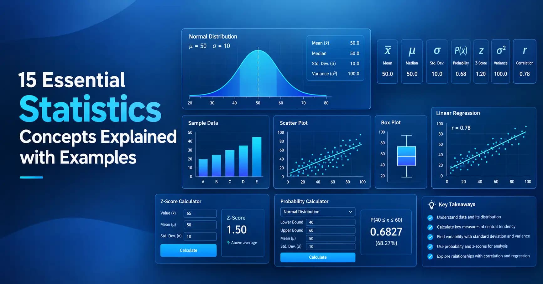
Statistics helps you make sense of data. It gives you ways to collect, organise, summarise, compare, and interpret numbers. You may use statistics to study exam results, sales, survey responses, sports records, business data, or results from a research study.
You don't need to know every statistics formula to get started. A good understanding of the main statistics concepts is more useful. Once you understand what a mean, median, standard deviation, probability, z-score, confidence interval, and p-value mean, many harder topics become easier to follow.
Statistics is often split into descriptive statistics and inferential statistics. Descriptive statistics summarise data, while inferential statistics use sample data to draw conclusions about a larger population.
Here are 15 essential statistical concepts, with simple examples and formulas where they help.
1. Population and Sample
A population is the full group you want to study. A sample is a smaller group taken from that population.
For example, suppose a university wants to know the average study time of all its students. All students at the university are the population. If researchers ask 500 students about their study time, those 500 students are the sample.
Using a sample can save time and money. In many studies, checking every member of a population isn't practical, so researchers use sample data to estimate population values.
A population value is called a parameter. A value calculated from a sample is called a statistic.
Example
Population: 20,000 university students
Sample: 500 university students
Sample mean study time: 16 hours per week
The 16-hour value is a sample statistic used to estimate the population mean.
2. Variables and Data Types
A variable is a characteristic that can take different values. Examples include age, height, income, test score, number of purchases, and favourite colour.
Variables can be numerical or categorical.
Numerical data uses numbers, such as:
- Age = 21
- Height = 175 cm
- Test score = 82
Categorical data places observations into groups, such as:
- Course = Mathematics
- Colour = Blue
- Payment type = Card
Knowing the type of data matters because not every statistical method works with every type of data. A variable can also be discrete, where values are counted, or continuous, where values can take any value within a range.
3. Mean
The mean is one of the most common measures of central tendency. It's often called the average.
To calculate the mean, add all the values and divide the total by the number of values.
Formula
Mean = Sum of all values ÷ Number of values
Example
Consider these five test scores:
12, 15, 15, 18, 20
Add them:
12 + 15 + 15 + 18 + 20 = 80
There are 5 scores.
Mean = 80 ÷ 5 = 16
So, the mean score is 16.
The mean works well when your data doesn't contain very large or very small values that can pull the average away from most observations.
4. Median
The median is the middle value after you put the data in order.
For an odd number of values, there is one middle value. For an even number of values, the median is the average of the two middle values.
Example
Data:
8, 12, 15, 17, 21
The middle value is 15, so the median is 15.
Now consider:
8, 12, 15, 17, 21, 30
The two middle values are 15 and 17.
Median = (15 + 17) ÷ 2 = 16
The median can be useful when your data has outliers.
For example, take these five salaries:
£25,000, £27,000, £29,000, £31,000, £150,000
The £150,000 value pushes the mean much higher, but the median stays at £29,000. This makes the median a useful measure for data with extreme values.
5. Mode
The mode is the value that appears most often in a data set.
Example
Data:
4, 5, 5, 6, 7, 5, 8
The number 5 appears three times.
Mode = 5
A data set can have one mode, more than one mode, or no mode.
The mode can also be used with categorical data. For example, if a survey asks people to choose a preferred colour and “blue” receives the most responses, blue is the mode.
6. Range and Interquartile Range
The range gives a quick measure of how spread out the data is.
Formula
Range = Maximum value - Minimum value
For:
12, 15, 15, 18, 20
the range is:
20 - 12 = 8
The interquartile range, or IQR, gives the spread of the middle 50% of the data.
Formula
IQR = Q3 - Q1
Here, Q1 is the first quartile and Q3 is the third quartile. Quartiles divide ordered data into four parts, while the median is the second quartile, or 50th percentile.
The IQR is useful when you want a measure of spread that is less affected by extreme values.
You'll often see range and IQR used with a box plot.
7. Variance
Variance measures how far data values vary from the mean. It uses the squared difference between each value and the mean.
For a sample, the formula is:
s² = Σ(x - x̄)² ÷ (n - 1)
Suppose your sample is:
12, 15, 15, 18, 20
We already found that the mean is 16.
The squared differences are:
- (12 - 16)² = 16
- (15 - 16)² = 1
- (15 - 16)² = 1
- (18 - 16)² = 4
- (20 - 16)² = 16
Total = 38
Sample variance:
38 ÷ 4 = 9.5
So, the sample variance is 9.5.
Variance is useful in statistics, but its squared units can make it harder to interpret directly. That's where standard deviation helps.
8. Standard Deviation
Standard deviation tells you how far data values tend to be from the mean. It is the square root of variance.
For the sample above:
Standard deviation = √9.5 ≈ 3.08
A small standard deviation means the values are close to the mean. A larger standard deviation means the values are more spread out.
Simple example
Data set A:
48, 49, 50, 51, 52
Data set B:
20, 35, 50, 65, 80
Both have a mean of 50, but data set B has much more spread. Its standard deviation is much larger.
This is why looking only at the mean isn't enough. Two data sets can have the same average but very different levels of variation.
9. Probability
Probability measures how likely an event is to happen. It ranges from 0 to 1, or from 0% to 100%.
A probability of 0 means an event cannot happen under the stated conditions. A probability of 1 means it must happen.
Formula
For equally likely outcomes:
Probability = Number of favourable outcomes ÷ Total number of possible outcomes
Example
A fair six-sided die has six possible results.
The probability of rolling a 4 is:
1 ÷ 6 ≈ 0.167
As a percentage:
16.7%
Probability plays a major role in inferential statistics because it helps us understand uncertainty and sample results.
10. Normal Distribution
The normal distribution is a common probability distribution with a bell-shaped curve. Values tend to cluster around the mean, with fewer observations appearing farther from the centre.
A normal distribution is described by its mean and standard deviation.
For example, suppose test scores follow a normal distribution with:
Mean = 70
Standard deviation = 10
Most scores would be near 70, while scores much lower or higher than 70 would be less common.
The normal distribution is widely used in statistics, probability, research, and data analysis. It also plays a key role in concepts such as z-scores, confidence intervals, and sampling distributions.
11. Z-Score
A z-score tells you how many standard deviations a value is from the mean.
Formula
z = (x - μ) ÷ σ
Where:
- x is the data value
- μ is the mean
- σ is the population standard deviation
Example
Suppose:
Mean = 70
Standard deviation = 10
Score = 85
Then:
z = (85 - 70) ÷ 10 = 1.5
The score of 85 is 1.5 standard deviations above the mean.
A negative z-score means the value is below the mean. A positive z-score means it is above the mean.
Z-scores make it easier to compare values from different data sets.
For example, an 85 in one exam and a 72 in another exam can't always be compared fairly by looking at the raw scores alone. Their z-scores can show how each result compares with its own distribution.
12. Sampling Distribution and Standard Error
A sampling distribution is the distribution of a statistic, such as the sample mean, across many possible samples of the same size.
This idea can feel strange at first. Imagine taking many random samples from the same population and calculating the mean of each sample. Those sample means create a sampling distribution.
The spread of sample means is called the standard error of the mean.
Formula
SE = σ ÷ √n
When the sample size increases, the standard error of the mean gets smaller. This means larger samples tend to give more precise estimates of the population mean.
This idea leads to the Central Limit Theorem, one of the key ideas behind many common statistical methods.
13. Confidence Interval
A confidence interval gives a range of values used to estimate a population parameter from sample data.
For example, a survey might estimate that the average response is 72, with a 95% confidence interval from 69 to 75.
A common form is:
Estimate ± Margin of Error
The exact calculation depends on factors such as sample size, variation, and the statistical method being used.
A 95% confidence level does not mean there is a 95% probability that a fixed population parameter is inside one particular calculated interval. In the repeated sampling view, about 95% of intervals made by the same method would contain the true parameter.
Why confidence intervals matter
A single sample estimate gives you one number. A confidence interval gives you an estimate along with information about its uncertainty.
That makes it much more useful when reporting research results.
14. Hypothesis Testing and P-Value
Hypothesis testing is a way to use sample data to assess a claim about a population. A test usually starts with a null hypothesis, which represents the claim being tested, and an alternative hypothesis.
Simple example
Suppose a company claims that its new training programme increases the average test score.
You could set up:
Null hypothesis: The programme does not increase the average score.
Alternative hypothesis: The programme increases the average score.
You then collect sample data and run an appropriate statistical test.
The p-value tells you how compatible the observed result is with the null hypothesis under the assumptions of the test. A smaller p-value provides stronger evidence against the null hypothesis. It does not tell you the probability that the null hypothesis is true.
A common significance level is 0.05, but the choice of significance level should be made as part of the study design rather than chosen only after seeing the result.
Hypothesis testing also involves the risk of errors. A Type I error occurs when a true null hypothesis is rejected. A Type II error occurs when a false null hypothesis is not rejected.
15. Correlation and Regression
Correlation measures the strength and direction of a linear relationship between two variables.
The Pearson correlation coefficient, usually written as r, ranges from -1 to +1. A value close to +1 shows a strong positive linear relationship, while a value close to -1 shows a strong negative linear relationship. A value near 0 shows little or no linear relationship.
Example
Suppose you compare:
- Hours studied
- Exam score
If students who study more hours tend to have higher scores, the two variables may have a positive correlation.
But correlation does not prove that one variable causes the other. Other factors may affect both variables.
Regression goes a step further. A linear regression model can describe the relationship between variables and can be used to estimate a value of one variable from another.
A simple regression equation can be written as:
ŷ = a + bx
Here, a is the intercept and b is the slope.
For example, you might use study hours as x and predicted exam score as y.
Regression is common in business analysis, research, forecasting, and data science. Statistical software and calculators can handle the calculations, but you still need to understand what the results mean.
How These Statistics Concepts Work Together
These concepts aren't separate boxes. They fit together.
Imagine you're studying exam results for 1,000 students.
You could start with a population of 1,000 students and select a sample. You might calculate the mean, median, and mode to describe the scores.
Next, you could measure variation with the range, IQR, variance, and standard deviation. A graph could help you see the shape of the data and whether the values look close to a normal distribution.
If you want to make a claim about all 1,000 students based on your sample, you move into inferential statistics. You may use a sampling distribution, standard error, confidence interval, or hypothesis test.
If you're studying the relationship between two variables, such as attendance and exam scores, correlation and regression may help describe that relationship.
That's the bigger picture of statistics:
Collect data → describe data → measure variation → study uncertainty → make inferences → examine relationships
Which Statistics Concept Should You Use?
The right method depends on the question you're asking.
| Question | Useful concept |
|---|---|
| What's the average? | Mean |
| What's the middle value? | Median |
| Which value occurs most often? | Mode |
| How spread out are the values? | Range, IQR, variance, standard deviation |
| How likely is an event? | Probability |
| How far is a value from the mean? | Z-score |
| What's a likely range for a population value? | Confidence interval |
| Does the sample provide evidence against a claim? | Hypothesis test |
| How are two variables related? | Correlation |
| Can one variable help estimate another? | Regression |
A statistics calculator can save time when the data set is large or when a formula has many steps. But the calculator only gives you the result. You still need to know which calculation fits the question and how to explain the answer.
Final Thoughts
Learning statistics becomes much easier when you understand the main ideas instead of trying to memorise every formula at once.
The mean, median, and mode help describe the centre of data. Range, IQR, variance, and standard deviation show how much the data varies. Probability and normal distributions help you work with uncertainty. Z-scores, sampling distributions, and confidence intervals help you compare values and estimate population results. Hypothesis testing helps assess claims, while correlation and regression help you study relationships between variables.
These 15 statistics concepts give you a solid base for statistics, data analysis, research, business studies, and data science. Once these ideas are clear, more advanced topics such as t-tests, ANOVA, chi-square tests, logistic regression, and statistical modelling become much easier to understand.